Next: Orthogonalization Convention Up: Crystallographic Diffraction Data Previous: Crystallographic Diffraction Data

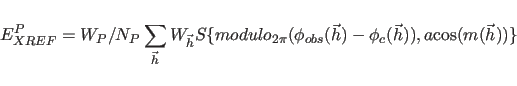
Crystallographic Target Functions

X-PLOR provides several possibilities for the effective energy $E_{XREF}$ . The selection of the target is specified by the TARGet keyword. There are seven possible choices: RESIdual, AB, F1F1, F2F2, E1E1, E2E2, and PACKing.

(13.1)

$\begin{displaymath} E_{XREF} = \left\{ \begin{array}{l} W_A/N_A \sum_{\vec{h}} ... ...}(\vec{h})^2]) \\ W_A (1- {\rm Pack} ) \end{array} \right. \end{displaymath}$

$\vec{h} = (h,k,l)$ is the Miller indices of the selected reflections, $F_{obs}$ is the observed structure factors, $F_{c}$ is the computed structure factors, $A_{obs}$ and $A_{c}$ are the real components, $B_{obs}$ and $B_{c}$ are the imaginary components of the structure factors,

is a normalization factor,

is a scale factor,

is an overall weight, $w_{\vec{h}}$ is the individual weights of the reflections,

s are normalized structure factors, and “Corr" is the standard linear correlation coefficient. The computation of the effective energy $E_{XREF}$ is accompanied by printing the unweighted

value

$\begin{displaymath} R = \frac{ \sum_{\vec{h}} \vert\vert F_{obs}(\vec{h})\vert... ...h})\vert\vert} { \sum_{\vec{h}} \vert F_{obs}(\vec{h})\vert } \end{displaymath}$

(13.2)

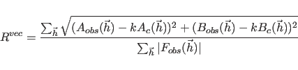
for the first choice in Eq. 13.1, the unweighted vector

value

$\begin{displaymath} R^{vec} = \frac{ \sum_{\vec{h}} \sqrt{(A_{obs}(\vec{h})-k... ...(\vec{h}))^2}} { \sum_{\vec{h}} \vert F_{obs}(\vec{h})\vert } \end{displaymath}$

(13.3)

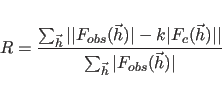
for the second choice, or the various correlation coefficients for the third to sixth choices. The

values are stored in the symbol $R, and the correlation coefficients are stored in the symbol $CORR. If the data are partitioned into a test and a working set (see Chapter 17), the corresponding values for the test set are stored in the symbols $TEST R and $TEST CORR.

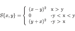
The selection of reflections is accomplished by the RESOlution and FWINdow statements (see below). “Corr" is defined through

$\begin{displaymath} {\rm Corr}[x \;, \; y] = \frac{<xy-<x><y»}{\sqrt{<x^2-<x>^2> \; <y^2-<y>^2>}} \end{displaymath}$

(13.4)

where the angle brackets denote a weighted ( $w_{\vec{h}}$ ) averaging over all selected Miller indices $\vec{h}$ . $F_{c}(\vec{h})$ is defined as

$\begin{displaymath} F_{c}(\vec{h})=F_{calc}(\vec{h})+F_{part}(\vec{h}) \end{displaymath}$

(13.5)

where $F_{part}(\vec{h})$ is “partial" structure factors that can be used to represent a “frozen" part of the molecule or bulk solvent contributions, and $F_{calc}(\vec{h})$ represents the structure factors that are computed from the current atomic model. $w_{\vec{h}}$ provides individual weights for each reflection $\vec h$ . The overall weight

relates $E_{XREF}^A$ to the other energy terms (see Section 4.6).

The normalized structure factors (s) are computed from the structure factors (s) by averaging the s in equal reciprocal volume shells within the specified resolution limits. The number of shells is specified by MBINs.

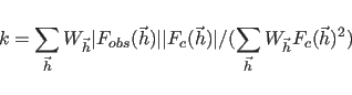
The purpose of the normalization factor (first and second choice in Eq. 13.1) is to make the weight approximately independent of the resolution range during SA-refinement. has been set to $N_A= \sum_{\vec h} W_{\vec h}\vert F_{obs}({\vec h})\vert^2$ . The scale factor in Eq. 13.1 is set to

$\begin{displaymath} k=\sum_{\vec h}W_{\vec h}\vert F_{obs}({\vec h})\vert\vert F... ...{\vec h})\vert / (\sum_{\vec h} W_{\vec h} F_{c}({\vec h})^2) \end{displaymath}$

(13.6)

unless it is set manually by the FFK statement. Eq. 13.6 is a necessary condition to minimize the residual.

The term $E_{XREF}^{P}$ represents phase restraints if is set to a nonzero number.

$\begin{displaymath} E_{XREF}^{P}=W_{P}/N_{P} \sum_{\vec h} W_{\vec{h}} S\{modu... ...obs}({\vec h})- {\phi}_{c}({\vec h})), a{\cos}(m({\vec h}))\} \end{displaymath}$

(13.7)

is a normalization factor set equal to the number of phase specifications occurring in the sum, $\phi_{obs}({\vec h})$ is the phase centroid obtained from mir or other methods (PHASe specifications; see Section 13.4), ${\phi}_{c}({\vec h})$ is the phase of the calculated structure factors $F_{c}(\vec{h})$ , $m({\vec h})$ is the individual figure of merit (FOM specifications; see Section 13.4), and $S\{x,y\}$ is a well function with harmonic “wells" given by

$\begin{displaymath} S\{x,y\}= \left\{ \begin{array}{lll} (x-y)^2 & \mbox{x $>$ ... ... x $<$ y} \\ (y+x)^2 & \mbox{-y $>$ x} \end{array}\right. \end{displaymath}$

(13.8)

This form of the effective energy $E_{XREF}^{P}$ ensures that the calculated phases are restrained to ${\phi}_{obs}({\vec h}){\pm}{\rm acos}(m({\vec h}))$ .

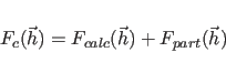
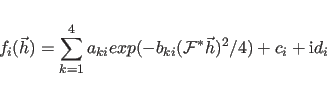
The structure factors ( $F_{calc}(\vec{h})$ ) of the atomic model are given by

(13.9)

$\begin{eqnarray*} F_{calc}(\vec{h})& = & \sum_{s \in S} \sum_{n \in NCS} \sum_... ...{\cal O}_{n}{\vec r_{i}} + \vec{t_n}) + \vec{t_{s}})) \nonumber \end{eqnarray*}$

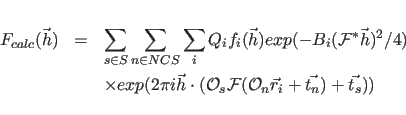
The first sum extends over all symmetry operators $({\cal O}_{s},\vec{t_{s}}; s \in S)$ composed of the matrix ${\cal O}_{s}$ representing a rotation and a vector $\vec{t_{s}}$ representing a translation. The second sum extends over all non-crystallographic symmetry operators $({\cal O}_{n},\vec{t_{n}}; n \in NCS)$ if they are present; otherwise only the identity transformation is used (see Chapter 18). The third sum extends over all unique atoms

of the system. The quantity $\vec {r_i}$ denotes the orthogonal coordinates of atom

in Å. ${\cal F}$ is the 3 ${\times}$ 3 matrix that converts orthogonal coordinates into fractional coordinates; ${\cal F}^{*}$ denotes the transpose of it. The columns of $\cal{F^*}$ are equal to the reciprocal unit cell vectors $\vec{a^*}, \vec{b^*}, \vec{c^*}$ .

is the occupancy for each atom.

is the individual atomic temperature factor for atom

. Both quantities correspond to the Q and B atom properties (Section 2.16), which can be read along with the atomic coordinates (see Section 6.1). The atomic scattering factors $f_{i}(\vec{h})$ are approximated by an expression consisting of four Gaussians and a constant

$\begin{displaymath} f_{i}(\vec{h}) = \sum^{4}_{k=1}a_{ki}exp(-b_{ki}({\cal F}^{*} {\vec h})^2 /4) + c_{i} + {\rm i} d_{i} \end{displaymath}$

(13.10)

The constants $a_{ki}$ and $b_{ki}$ are specified in the SCATter statement and can be obtained from the International Tables for Crystallography (Hahn, 1987). The term ${\rm i} d_i$ denotes an imaginary constant that can be used to model anomalous scattering. Eq. 13.9 represents the space-group general form of the “direct summation" formula, which is used to compute the structure factors. The fast Fourier transformation (FFT) method consists of computing $F_{calc}(\vec{h})$ by numerical evaluation of the atomic electron density on a finite grid followed by an FFT. The FFT method provides a way to speed up the calculation. The METHod statement can be used to switch between the FFT method and the direct summation method.

An approximation is used to reduce the computational requirements when multiple evaluations of Eq. 13.1 are required. The approximation involves not computing $F_{calc}(\vec{h})$ and its first derivatives at every dynamics or minimization step. The first derivatives are kept constant until any atom has moved by more than $\Delta_{F}$ (TOLErance in xrefin statement) relative to the position at which the derivatives were last computed. At that point, all derivatives are updated. Typically, $\Delta_{F}$ is set to 0.2 Å for dynamics and to 0-0.05 Å for minimization.

The PACKing target is defined for evaluating the likelihood of packing arrangements of the search model and its symmetry mates in the crystal (Hendrickson and Ward, 1976). A finite grid that covers the unit cell of the crystal is generated. The grid size is specified through the GRID parameter in the xrefin FFT statement. All grid points are marked that are within the van der Waals radii around any atom of the search model and its symmetry mates. The number of marked grid points represents the union of the molecular spaces of the search model and its symmetry mates. Maximization of the union of molecular spaces is equivalent to minimization of the overlap. Thus, an optimally packed structure has a maximum of the packing function. “Pack" in Eq. 13.1 contains the ratio of the number of marked grid points to the total number of grid points in the unit cell. For instance, a value of 0.6 means 40% solvent contents. $E_{XREF}=W_A (1- {\rm Pack} )$ is then set to 0.4 if .

For further reading on the crystallographic target functions in X-PLOR, see Brünger (1990,1988,1989).

Xplor-NIH 2024-09-13