
| bit | Xplor-NIH | VMD-XPLOR |
|---|
|
| Xplor-NIH home Documentation |
Next: Cutoffs Up: NMR Back-calculation Refinement Previous: Analytical Expression for the
The
 Energy Term
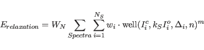
Once the NOESY spectrum and its gradient are calculated, the
relaxation energy
where
The individual error estimates
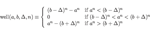
Values for the exponents of ![]() and
and ![]() (Eqs. 39.9
and 39.10) correspond to the refinement of the residual in X-ray
crystallography. These values tend to put a high weight on the
large intensities, resulting in a bad fit of intensities for which
the calculated value is too small. Following a suggestion
by James et al. (1991), use
(Eqs. 39.9
and 39.10) correspond to the refinement of the residual in X-ray
crystallography. These values tend to put a high weight on the
large intensities, resulting in a bad fit of intensities for which
the calculated value is too small. Following a suggestion
by James et al. (1991), use ![]() and
and
![]() . A value of
. A value of ![]() results in the refinement of the
results in the refinement of the
![]() value directly, instead of the residual. The discontinuity of the
gradient may lead to instabilities during the refinement.
value directly, instead of the residual. The discontinuity of the
gradient may lead to instabilities during the refinement.
In addition to the overall weight ![]() , individual weights
, individual weights ![]() can be applied to each term in the sum in Eqs. 39.9
and 39.12, e.g.,
in order to increase the relative weight of the small intensities.
(It should be noted that this is achieved already by setting
can be applied to each term in the sum in Eqs. 39.9
and 39.12, e.g.,
in order to increase the relative weight of the small intensities.
(It should be noted that this is achieved already by setting ![]() in Eq. 39.9.)
The scheme
in Eq. 39.9.)
The scheme
![]() corresponds to a
common weighting scheme
used in crystallography if experimental
corresponds to a
common weighting scheme
used in crystallography if experimental ![]() values are unreliable
or unavailable.
In the NMR case, however, there is no theoretical justification
for this weighting scheme. (In crystallography, the statistical error
values are unreliable
or unavailable.
In the NMR case, however, there is no theoretical justification
for this weighting scheme. (In crystallography, the statistical error
![]() of an intensity measurement
of an intensity measurement ![]() is
is
![]() .)
The weights are scaled such that
.)
The weights are scaled such that ![]() .
.
The calibration factor between observed and back-calculated
intensities is determined simply as the ratio of the sums of all
calculated and observed intensities:
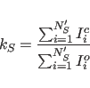 |
(39.11) |
Next: Cutoffs Up: NMR Back-calculation Refinement Previous: Analytical Expression for the Contents Index