
| bit | Xplor-NIH | VMD-XPLOR |
|---|
|
| Xplor-NIH home Documentation |
Next: Syntax of the Dynamics Up: Rigid-Body Coordinate Space Previous: Initialization
Iteration
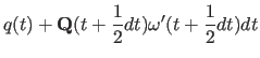
After initialization, the center-of-mass variables are integrated using the three-step Verlet method: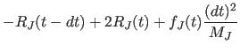 |
(11.24) | ||
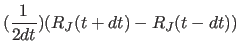 |
(11.25) |
Friction terms are embedded in the force
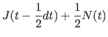
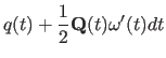
The integration of rotational variables uses a different central difference
expansion. The algorithm begins with the advancement of the Euler-Cayley
parameters by ![]() , using the following four steps:
, using the following four steps:
 |
(11.26) | ||
| (11.27) | |||
| (11.28) | |||
 |
 |
(11.29) |
Here
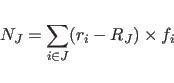 |
(11.30) |
 |
 |
(11.31) | |
 |
 |
(11.32) | |
 |
 |
(11.33) | |
 |
(11.34) |
The velocities of individual atoms, which are necessary for the friction evaluation, are determined using the angular velocities of the rigid bodies. The velocity due to rotation alone is determined in the body frame, then transformed into the lab frame and added to the translational velocity of the center of mass:
![\begin{displaymath}
v_i(t)=V_J(t)+{\bf A_J}^{-1}\left[\begin{array}{c}
z^B_{i}\o...
...\
y^B_{i}\omega^B_{x}-x^B_{i}\omega^B_{y}
\end{array} \right]
\end{displaymath}](img370.png) |
(11.35) |
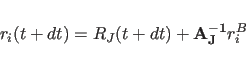 |
(11.36) |
The rigid-body dynamics routine can be run in one of three modes:
FREE, LANGevin, or TCOUpling. The FREE mode simply allows frictionless
dynamics, the LANGevin mode adds friction- and bath-dependent random
forces, and TCOUpling uses the method of
Berendsen et al. (1984). The coordinates (and velocities)
are affected by using a nonzero friction coefficient in the
Langevin dynamics algorithm with zero random forces. The friction
coefficient
is computed by the program from the equation
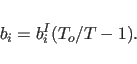 |
(11.37) |
If the simulation involves light rigid groups such as water molecules, it is recommended that a time step on the order of .25 fsec be used. For heavier groups, time steps as large as 20 or 30 fsec are adequate.
Next: Syntax of the Dynamics Up: Rigid-Body Coordinate Space Previous: Initialization Contents Index